Author: hmnjr0lnuhzp

  • bmp180

    English | 简体中文 | 繁體中文 | 日本語 | Deutsch | 한국어

    LibDriver BMP180

    MISRA API License

    The BMP180 is the function compatible successor of the BMP085, a new generation of high precision digital pressure sensors for consumer applications.The ultra-low power, low voltage electronics of the BMP180 is optimized for use in mobile phones, PDAs, GPS navigation devices and outdoor equipment. With a low altitude noise of merely 0.25m at fast conversion time, the BMP180 offers superior performance. The IIC interface allows for easy system integration with a microcontroller.The BMP180 is based on piezo-resistive technology for EMC robustness, high accuracy and linearity as well as long term stability.

    LibDriver BMP180 is a full-featured driver of BMP180 launched by LibDriver.It provides temperature, pressure reading and mode setting functions and so on. LibDriver is MISRA compliant.

    Table of Contents

    Instruction

    /src includes LibDriver BMP180 source files.

    /interface includes LibDriver BMP180 IIC platform independent template.

    /test includes LibDriver BMP180 driver test code and this code can test the chip necessary function simply.

    /example includes LibDriver BMP180 sample code.

    /doc includes LibDriver BMP180 offline document.

    /datasheet includes BMP180 datasheet.

    /project includes the common Linux and MCU development board sample code. All projects use the shell script to debug the driver and the detail instruction can be found in each project’s README.md.

    /misra includes the LibDriver MISRA code scanning results.

    Install

    Reference /interface IIC platform independent template and finish your platform IIC driver.

    Add the /src directory, the interface driver for your platform, and your own drivers to your project, if you want to use the default example drivers, add the /example directory to your project.

    Usage

    You can refer to the examples in the /example directory to complete your own driver. If you want to use the default programming examples, here’s how to use them.

    example basic

    #include "driver_bmp180_basic.h"
    
    uint8_t res;
    uint32_t i;
    float temperature;
    uint32_t pressure;
    
    res = bmp180_basic_init();
    if (res != 0)
    {
        return 1;
    }
    
    ...
    
    for (i = 0; i < 3; i++)
    {
        bmp180_interface_delay_ms(1000);
        res = bmp180_basic_read((float *)&temperature, (uint32_t *)&pressure);
        if (res != 0)
        {
            (void)bmp180_basic_deinit();
    
            return 1;
        }
        bmp180_interface_debug_print("bmp180: temperature is %0.2fC.\n", temperature);
        bmp180_interface_debug_print("bmp180: pressure is %dPa.\n", pressure);
        
        ...
            
    }
    
    ...
    
    (void)bmp180_basic_deinit();
    
    return 0;

    Document

    Online documents: https://www.libdriver.com/docs/bmp180/index.html.

    Offline documents: /doc/html/index.html.

    Contributing

    Please refer to CONTRIBUTING.md.

    License

    Copyright (c) 2015 – present LibDriver All rights reserved

    The MIT License (MIT)

    Permission is hereby granted, free of charge, to any person obtaining a copy

    of this software and associated documentation files (the “Software”), to deal

    in the Software without restriction, including without limitation the rights

    to use, copy, modify, merge, publish, distribute, sublicense, and/or sell

    copies of the Software, and to permit persons to whom the Software is

    furnished to do so, subject to the following conditions:

    The above copyright notice and this permission notice shall be included in all

    copies or substantial portions of the Software.

    THE SOFTWARE IS PROVIDED “AS IS”, WITHOUT WARRANTY OF ANY KIND, EXPRESS OR

    IMPLIED, INCLUDING BUT NOT LIMITED TO THE WARRANTIES OF MERCHANTABILITY,

    FITNESS FOR A PARTICULAR PURPOSE AND NONINFRINGEMENT. IN NO EVENT SHALL THE

    AUTHORS OR COPYRIGHT HOLDERS BE LIABLE FOR ANY CLAIM, DAMAGES OR OTHER

    LIABILITY, WHETHER IN AN ACTION OF CONTRACT, TORT OR OTHERWISE, ARISING FROM,

    OUT OF OR IN CONNECTION WITH THE SOFTWARE OR THE USE OR OTHER DEALINGS IN THE

    SOFTWARE.

    Contact Us

    Please send an e-mail to lishifenging@outlook.com.

    Visit original content creator repository https://github.com/libdriver/bmp180
  • NapicuWebGame-Pong

    NapicuWebGame – Pong

    Upozornění

    • Hra není optimalozováná pro výkon!
    • Nedoporučuje se hostovat hru na slabém hostingu!
    • Doporučujeme hostovat pouze na localhostu!

    Hra pro více hráčů

    • Hráč 1 pošle kód Hráči 2, který ho následně zadá do kolonky Připojit se

    • Jestli kód opsal správně půjde odestal pozvánka

    • Informace

      • Pozvánka můžete poslat pouze hráči, který ještě žádnou pozvánku nedostal
      • Nelze pozvat hráče, který již hraje
      • Hra se automaticky ukončí, když 1 z hráčů odpojí hru. Druhému hráči se automaticky vygeneruje nový kód

    Instalace

    • instalace balíčku
    npm i
    
    • .env – port na kterém aplikace poběží
    PORT=8080
    

    Celé fungování hry

    • Při připojení do hry se automaticky vygeneruje základní informace o hráči ve funkci GetNewRoom()
      • ActivityRoom = Room id ve které se uživatel nachází
      • Player = Ve hře – Rozlišení zda je hráč “Hrac1” nebo “Hrac1”
    • Při requestu
      • Kontroluje se zda zadané room id není room id zadavatele
      • Kontroluje se zda v roomce není 2 a více hráčů
      • Uloží se PlayersRequest Map() id hráče který chce být pozván a id hráče, který vytvořil pozvánku
      • Kontroluje se hráč v roomce nemá již ( z PlayersRequest ) poslaný request od jiného hráče
      • Zda je vše v pořádku pošle se invite hráči v roomce
      • Také se pošle zadavateli potvrzení o poslání requestu hráči
    • Při acceptu
      • Kontroluje se zda Hráč který poslal pozvánku se neodpojil
      • Odstraní se id z PlayersRequest
      • Hráč který vytvořil pozvánku se připojí k hráči ( “Majitele roomky” )
      • Nastaví se socket.Player – Hrac1 – Majitel roomky
      • Dále se nastaví Hráči2 ActivityRoom (id roomky)
      • Připojí se k Hraci1
      • Do roomky se pošle emit Ready
      • Zda je vše v pořádku pošle se emit PingStart
    • Při PingStart
      • Kontroluje se zda hráči i nejsou v Players (Map())
      • Také se kontroluje zda Koule s id roomky není v Balls (Map())
      • Zda je hráč Hrac1 dostane souřadnice x: 100
      • Zda je hráč Hrac2 dostane souřadnice x: 1700
      • Dále se vytvoří Player (class)
      • Dále se vytvoří Ball (class)
      • Poté se uloží do Players (Map()) id hráče a všechny údaje o hráči
      • Do Balls se uloží id roomky a všechny další údale o ball
      • Následuje setInterval funkce která opakuje Render
    • Render function
      • Spouští se funkce Koule.Render(), která hýbe koulí
      • Dále se odesílá do roomky údaje o kouli
      • Poté se spouští funkce PlayerPush, která odesílá do roomky údaje o hráčích, kteří jsou v dané roomce
      • Funkce Render se opakuje každých 33ms (Z tohoto důvodu není doporučené hostovat tuto appku)
    • Při START
      • Odešle se do roomky emit o STARTU hry
      • U klienta se spustí funkce StartRender(), které spustí funkci requestAnimationFrame() která se opakuje podle frekvence monitoru a podle toho zda je Game.Player = true. Jestli je Game.Player = false, canvas se nebude renderovat
      • Také se spustí funkce Start(), která upraví prostředí pro hraní
    • Game.Render() function
      • Začne renderovat Background, ,Player Ball,
      • Kontroluje zda MoveKey.Up nebo MoveKey.Down je true
      • Zda je MoveKey.Up nebo MoveKey.Down true pošle se emit serveru PlayerMoveUp nebo PlayerMoveDown
    • Při PlayerMoveUp
      • Hráč se posune nahorů
    • Při PlayerMoveDown
      • Hráč se posune dolů
    • Player.Render() function
      • Spustí se funkce Player.Get(), která pošle emit PlayerUpdate který na serveru hýbe hráčem
      • Zda dostane PlayerMove uloží se u klienta údaje o hráčovi
      • Poté se už renderuje podle údajů u klienta
    • Ball.Render() function
      • Spustí se funkce Ball.get(), která získá údaje o kouli a uloží se u klienta
      • Poté se spustí funkce Ball.MainRender(), která renderuje podle údajů u klienta
    • Při disconnect
      • Stopne se intervatFun ( setInterval() )
      • Vymaže se Balls s id socketu ze kterého se uživatel odpojil
      • Vymažou se údaje o hráčovi z Players
      • Spustí se funkce PlayerLeftGame()

    Další funkce

    • PlayerPush() posílá do roomky údaje o hráčích které jsou v dané roomce
    • randomString() vygeneruje se hex string o délce 5
    • GETPlayersDataSocketRoom() vrátí údaje hráčů v roomce
    • GetRoomPlayers() vrátí socket id hráčů v roomce
    • GetPlayerByRoom() vrátí socket id prvního hráče v roomce
    • OnePlayerLeftGame() Pošle hráči, který zůstal v roomce emit PlayerLeft a spustí funkci GetNewRoom()
    • GetNewRoom() vygeneruje základní údaje (roomName, Player)

    Použité balíčky

    • crypto@1.0.1
    • dotenv@8.2.0
    • ejs@3.1.6
    • express@4.17.1
    • nodemon@2.0.7
    • socket.io@4.0.1

    Visit original content creator repository
    https://github.com/Numax-cz/NapicuWebGame-Pong

  • SSD1306TUR

    SSD1306TUR

    SSD1306TUR is a library that allows you to write any Turkish char on SSD1306 monochrome oled displays freely. Based on Adafuit’s SSD1306 oled Display driver can be found on here. Please be sure this lib is present in your system before use this lib.

    If you find any problem or bug on this library, please use Issues feature on github or contact me on my web page devrelerim.com.

    You can follow me on:

    Basic Usage

    include header file

    #include <Wire.h>
    #include <SSD1306TUR.h>

    You should use fonts placed TrFonts directory in this repository by including like this:

    #include "TrFonts/FreeSansBold12pt7bTR.h"

    define LCD specs fit your screen:

    #define SCREEN_WIDTH 128
    #define SCREEN_HEIGHT 64
    #define SCREEN_ADDRESS 0x3C

    initiate the object as any name you want, I choose display

    SSD1306TUR display(SCREEN_WIDTH, SCREEN_HEIGHT, &Wire);

    begin screen

    display.begin(SSD1306_SWITCHCAPVCC, SCREEN_ADDRESS)

    set text params and just write any Turkish letter by print, println or write functions.

    display.setTextColor(SSD1306_WHITE);
    display.clearDisplay();
    display.setTextSize(1);
    display.setFont(&FreeSansBold12pt7bTR);
    display.setCursor(20, 22);
    display.print("Türkçe");
    display.display(); 

    Dependencies

    Download

    You can download this on

    • Github
    • Arduino Library Manager
    • PlatformIO Libraries

    Available Fonts

    • FreeSansBold12pt7bTR.h

    more fonts will be added in the future, If you interested in creating new fonts to help this repository please feel free to contact me hakkanr@gmail.com

    Visit original content creator repository
    https://github.com/HakkanR/SSD1306TUR

  • sandboxrepo

    Sandbox Repository

    Repository for various packages (used by spkg, a package manager.)
    This is a special repo in that it supports *nix-In-A-Box apps, like LibTerm and OpenTerm.
    The tool used to download packages from this repo will be similar to apt, using a Release file. See here.
    This repo is still work in progress, so use at your own risk.

    – User-submitted software –

    (You are strongly recommended to submit your software under a OSI-approved license, like the GPLv3 or MIT License.)

    Users can submit a pull request with the command in this form:

    For OpenTerm, tarball(tar -czvf) the whole .prideland command folder and submit a pull request, with a appropiate description in the metadata.plist file.
    Because spkg in OpenTerm relies on a RELEASE file, your package name should also be added there.

    For Libterm (spkg is working somewhat), zip the .py command (stored in ~/Library/scripts) by itself and submit a pull request. (Make sure its not nested in another folder!)
    If you had not installed zip yet, install with “package install zip”. (The zip command from @ColdGrub1384’s repo is not working.
    I will upload a (fairly) basic zip program here for Libterm soon, so run [spkg -i zip2] to install.)
    spkg in Libterm is more advanced, and will automatically get the package list from the Github REST API
    so a RELEASE file is not needed. Just upload the package and everybody can download it right away.

    •New repositories!!!•

    The whole point of spkg was to enable external repository support for pulling software.
    Now you can, too! Create a RELEASE file in your repo in the Master branch under a “openterm” or a “libterm” folder, whichever platform you want to support. The RELEASE file is crucial as it contains a list of all programs in the repo.
    (Particularly important because users will not know what programs they can install.)

    Credits/Licenses

    The credits for each script are stored in a plaintext contained in the same folder where that author’s package is.
    Be careful to check the credits file first as this repository has more than one license for all its packages if you want to clone or fork the repo.

    Visit original content creator repository
    https://github.com/ongyx/sandboxrepo

  • pasticciotto

    Pasticciotto

    TravisCI Say Thanks!

    Pasticciotto

    What is this?

    Pasticciotto is a virtual machine which can be used to obfuscate code. It was developed for the PoliCTF 17 as a reversing challenge.

    The key feature is its opcode “shuffling”: their actual values are determined by a password. (More in IMPLEMENTATION.md)

    I wanted to experiment with VM obfuscation since it was a topic that caught my attention while reversing challenges for various CTFs. So, I decided to write one from scratch in order to understand better how instruction set architectures are implemented!

    The design and the implementation behind Pasticciotto are not state-of-the-art but hey, it works! 😀

    Why “Pasticciotto”?

    In Italian, “Pasticciotto” has two meanings!

    The first one is “little mess” which perfectly describes how I put up this project. The second one is a typical dessert from Southern Italy, Salento! It’s filled with cream! Yum!

    Quick start

    You can use pasticciotto in your own binary! It’s easy to do!

    Assemble!

    Let’s say you want to run this C code into pasticciotto:

    void main() {
        uint16_t i, a, b;
        a = 0;
        b = 0x10;
    
        for (i = 0; i < b; i++) {
            a += b;
        }
        return;
    }

    It can be translated into this pasticciotto‘s assembly snippet:

    $ cat example.pstc
    def main:
    movi r0, 0x0  # a
    movi r1, 0x10 # b
    movi s1, 0x0  # i
    loop:
    addr r0, r1
    addi s1, 1
    cmpr s1, r1
    jpbi loop
    shit
    

    Let’s assemble it with key HelloWorld:

    $ python3 assembler.py HelloWorld example.pstc example_assembled.pstc
    

    Now we are ready to embed the VM in a .c program:

    #include "vm/vm.h"
    #include <fstream>
    #include <stdint.h>
    #include <stdio.h>
    #include <stdlib.h>
    
    int main(int argc, char *argv[]) {
        /*
        In order to create the bytecode for pasticciotto, you can use
        the assembler in the assembler/ directory. You can include it with
        `xxd -i example_assembled.pstc`
        */
        unsigned char example_assembled_pstc[] = {
        0x32, 0x00, 0x00, 0x00, 0x32, 0x01, 0x10, 0x00, 0x32, 0x05, 0x00, 0x00,
        0xaf, 0x01, 0xcf, 0x05, 0x01, 0x00, 0x8b, 0x51, 0xc5, 0x0c, 0x00, 0x0c
        };
        unsigned int example_assembled_pstc_len = 24;
        unsigned char key[] = {
        0x48, 0x65, 0x6c, 0x6c, 0x6f, 0x57, 0x6f, 0x72, 0x6c, 0x64, 0x0a
        };
    
    
        puts("I should try to eat a pasticciotto...\n");
        VM vm(key, example_assembled_pstc, example_assembled_pstc_len);
        vm.run();
        return 0;
    }

    That’s it!

    Accessing to the VM’s sections and registers

    The VM data / code / stack sections are represented through the VMAddrSpace object. It is defined here. The registers are in a uint16_t array in the VM object defined here.

    void foo() {
        // creating the VM with some code
        VM vm(key, code, codelen);
    
        // accessing the data section
        printf("First data byte: 0x%x", VM.addrSpace()->getData()[0]);
        // accessing the code section
        printf("First code byte: 0x%x", VM.addrSpace()->getCode()[0]);    
        // accessing the stack section
        printf("First stack byte: 0x%x", VM.addrSpace()->getStack()[0]);
        // accessing the IP register
        printf("The IP is: 0x%x", VM.regs(IP));
        return;
    }

    What about the challenge?

    You can find the client and the server under the polictf/ directory. I have also written a small writeup. Check it out!

    Compiling

    Requisites

    1. CMake

    Quick start

    mkdir build
    cd build
    cmake ..
    # or, if you want debug info:
    # cmake -DPASTICCIOTTO_DEBUG=On ..
    make
    

    CMake targets

    Target name Description
    pasticciotto-emulator Builds pasticciotto’s emulator
    polictf Builds PoliCTF’s client and server
    polictf-client Builds PoliCTF’s client
    polictf-server Builds PoliCTF’s server
    pasticciotto-tests Builds pasticciotto’s test executable.

    If the PASTICCIOTTO_DEBUG flag is passed to cmake during the configuration phase, the targets will be compiled with debug symbols and additional debug information.

    Implementation details

    Check out the file IMPLEMENTATION.MD to understand how the VM works and which operations it can do! Watch out for some spoilers if you haven’t completed the challenge though!

    Contributions

    I wanted to polish the VM even more but I haven’t got the time to do it. There are rough edges for sure!

    Any contribution is very welcome! Feel free to open issues and pull requests!

    License

    Copyright 2017 Giulio De Pasquale
    
    Permission is hereby granted, free of charge, to any person obtaining a copy of this 
    software and associated documentation files (the "Software"), to deal in the Software 
    without restriction, including without limitation the rights to use, copy, modify, merge, 
    publish, distribute, sublicense, and/or sell copies of the Software, and to permit persons 
    to whom the Software is furnished to do so, subject to the following conditions:
    
    The above copyright notice and this permission notice shall be included in all copies or 
    substantial portions of the Software.
    
    THE SOFTWARE IS PROVIDED "AS IS", WITHOUT WARRANTY OF ANY KIND, EXPRESS OR IMPLIED, 
    INCLUDING BUT NOT LIMITED TO THE WARRANTIES OF MERCHANTABILITY, FITNESS FOR A PARTICULAR 
    PURPOSE AND NONINFRINGEMENT. IN NO EVENT SHALL THE AUTHORS OR COPYRIGHT HOLDERS BE LIABLE 
    FOR ANY CLAIM, DAMAGES OR OTHER LIABILITY, WHETHER IN AN ACTION OF CONTRACT, TORT OR 
    OTHERWISE, ARISING FROM, OUT OF OR IN CONNECTION WITH THE SOFTWARE OR THE USE OR OTHER 
    DEALINGS IN THE SOFTWARE.
    
    Visit original content creator repository https://github.com/peperunas/pasticciotto
  • gatling-sentry-extension

    gatling-sentry-extension

    gatling-sentry-extension is the one that can easily send gatling logs to sentry. Gatling is the powerful tool to check application’s performance, but it is hard to check what kind of errors occur during the test. So, this extension help you check error logs with Sentry.(https://sentry.io/welcome/)
    This extension is made based on Akka framework, when the start gatling test, it should make Actor system for gatling-sentry-extension. I will explain more detaily below section.

    This extension can send those logs to Sentry.

    • Gatling http response
    • All string logs that you want

    Installation

    If you want to use, need to add the dependency in your build.sbt

    "com.github.allenkim80" % "gatling-sentry-extension_2.11" % "0.1.17"
    

    Usage

    Create actor system for sentry-extension

    // You need to make gatling simulation project.
    
    class SetnryTestSimulation extends Simulation {
    
      // Start extension
      startSentry()
    
      val scn = scenario("Sentry")
        .exec(
          http("/endpoint")
            .get("/endpoint")
            .transformResponse {case response if response.isReceived => sendSentryLog(response, List("Error1", "message")}  
        ).exec()
        .exec(sentry("").sendStringLogByAction("test2", "message"))
        .pause(3)
     
     def createHttpProtocol() : HttpProtocolBuilder = {
        http
          .baseURL("http://server-address")
          .acceptHeader("*/*")
          .headers(Map(
            "Content-Type" -> "application/json"
          ))
          .disableWarmUp
      }
     
     def sendSentryLog(response: Response, validErrors:List[String], message:String = "") = {
        val resultObject = new JsonParser().parse(response.body.string).getAsJsonObject.get("result")
    
        resultObject match {
          case result if result != null && result.getAsString == "true" => /* do nothing */
          case _ =>
            val reasonObject = new JsonParser().parse(response.body.string).getAsJsonObject.get("reason")
    
            if (!validErrors.contains(reasonObject.getAsString)) {
              sentry("").sendHttpLog(response)
            }
        }
        response
      }
    
      // start gatling simulation
      setUp(scn.inject(rampUsers(2) over (1 minute))).protocols(createHttpProtocol())
    
      // stop extension
      stopSentry()
    
    }
    

    Visit original content creator repository
    https://github.com/allenkim80/gatling-sentry-extension

  • anomalytics

    Anomalytics

    Your Ultimate Anomaly Detection & Analytics Tool

    pre-commit.ci status Code style: black Imports: isort mypy checked CI - Build CI - Code Quality CI - Automated Testing License: MIT Documentation PyPi

    Introduction

    anomalytics is a Python library that aims to implement all statistical methods for the purpose of detecting any sort of anomaly e.g. extreme events, high or low anomalies, etc. This library utilises external dependencies such as:

    anomalytics supports the following Python’s versions: 3.10.x, 3.11.x, 3.12.0.

    Installation

    To use the library, you can install as follow:

    # Install without openpyxl
    $ pip3 install anomalytics
    
    # Install with openpyxl
    $ pip3 install "anomalytics[extra]"

    As a contributor/collaborator, you may want to consider installing all external dependencies for development purposes:

    # Install bandit, black, isort, mypy, openpyxl, pre-commit, and pytest-cov
    $ pip3 install "anomalytics[codequality,docs,security,testcov,extra]"

    Use Case

    anomalytics can be used to analyze anomalies in your dataset (both as pandas.DataFrame or pandas.Series). To start, let’s follow along with this minimum example where we want to detect extremely high anomalies in our dataset.

    Read the walkthrough below, or the concrete examples here:

    Anomaly Detection via the Detector Instance

    1. Import anomalytics and initialise our time series of 100_002 rows:

      import anomalytics as atics
      
      df = atics.read_ts("./ad_impressions.csv", "csv")
      df.head()
                     datetime	    xandr	      gam	    adobe
      0	2023-10-18 09:01:00	52.483571	71.021131	35.681915
      1	2023-10-18 09:02:00	49.308678	73.651996	60.347246
      2	2023-10-18 09:03:00	53.238443	65.690813	48.120805
      3	2023-10-18 09:04:00	57.615149	80.944393	59.550775
      4	2023-10-18 09:05:00	48.829233	76.445099	26.710413
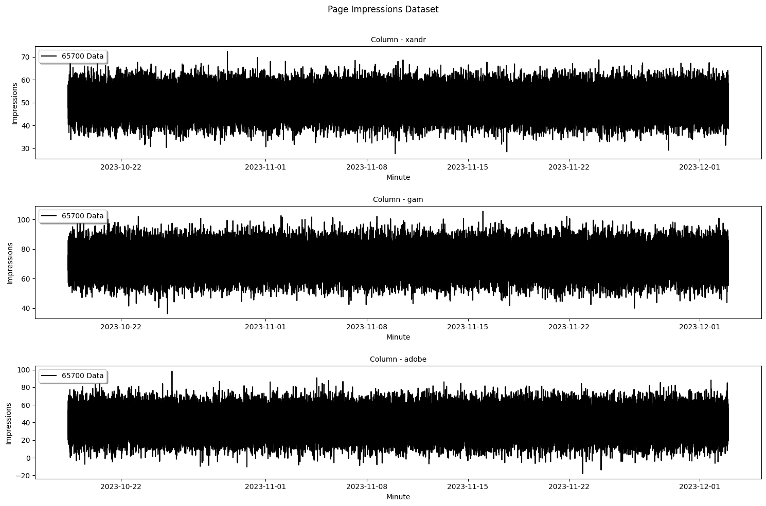
    2. Initialize the needed detector object. Each detector utilises a different statistical method for detecting anomalies. In this example, we’ll use POT method and a high anomaly type. Pay attention to the time period that is directly created where the t2 is 1 by default because “real-time” always targets the “now” period hence 1 (sec, min, hour, day, week, month, etc.):

      pot_detector = atics.get_detector(method="POT", dataset=ts, anomaly_type="high")
      
      print(f"T0: {pot_detector.t0}")
      print(f"T1: {pot_detector.t1}")
      print(f"T2: {pot_detector.t2}")
      
      pot_detector.plot(ptype="line-dataset-df", title=f"Page Impressions Dataset", xlabel="Minute", ylabel="Impressions", alpha=1.0)
      T0: 42705
      T1: 16425
      T2: 6570

      Ad Impressions Dataset

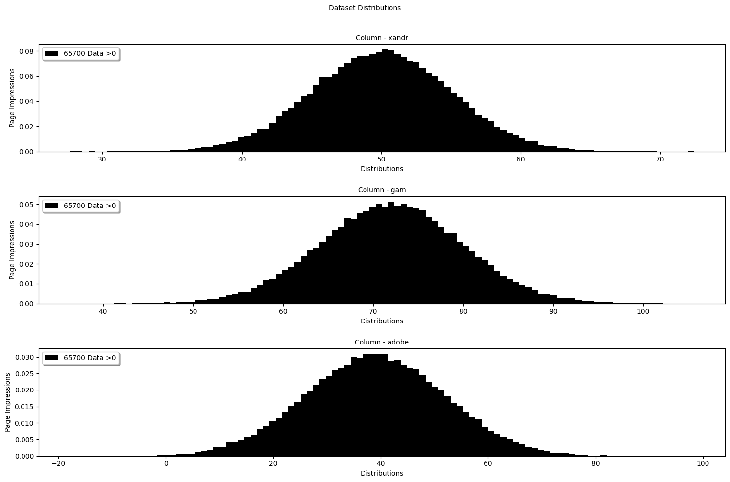
    3. The purpose of using the detector object instead the standalone is to have a simple fix detection flow. In case you want to customize the time window, we can call the reset_time_window() to reset t2 value, even though that will beat the purpose of using a detector object. Pay attention to the period parameters because the method expects a percentage representation of the distribution of period (ranging 0.0 to 1.0):

      pot_detector.reset_time_window(
          "historical",
          t0_pct=0.65,
          t1_pct=0.25,
          t2_pct=0.1
      )
      
      print(f"T0: {pot_detector.t0}")
      print(f"T1: {pot_detector.t1}")
      print(f"T2: {pot_detector.t2}")
      
      pot_detector.plot(ptype="hist-dataset-df", title="Dataset Distributions", xlabel="Distributions", ylabel="Page Impressions", alpha=1.0, bins=100)
      T0: 65001
      T1: 25001
      T2: 10000

      Ad Impressions Hist

    4. Now, we can extract exceedances by giving the expected quantile:

      pot_detector.get_extremes(0.95)
      pot_detector.exeedance_thresholds.head()
              xandr	      gam	    adobe	           datetime
      0	58.224653	85.177029	60.362306	2023-10-18 09:01:00
      1	58.224653	85.177029	60.362306	2023-10-18 09:02:00
      2	58.224653	85.177029	60.362306	2023-10-18 09:03:00
      3	58.224653	85.177029	60.362306	2023-10-18 09:04:00
      4	58.224653	85.177029	60.362306	2023-10-18 09:05:00
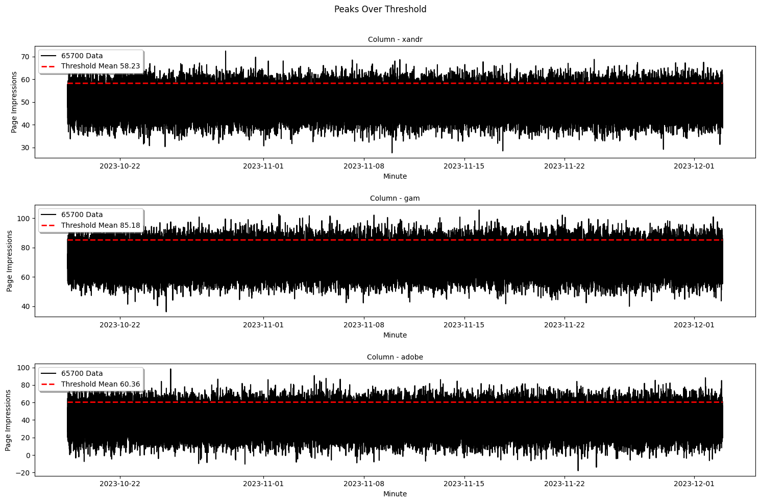
    5. Let’s visualize the exceedances and its threshold to have a clearer understanding of our dataset:

      pot_detector.plot(ptype="line-exceedance-df", title="Peaks Over Threshold", xlabel="Minute", ylabel="Page Impressions", alpha=1.0)

      Exceedance-POT

    6. Now that we have the exceedances, we can fit our data into the chosen distribution, in this example the “Generalized Pareto Distribution”. The first couple rows will be zeroes which is normal because we only fit data that are greater than zero into the wanted distribution:

      pot_detector.fit()
      pot_detector.fit_result.head()
          xandr_anomaly_score gam_anomaly_score   adobe_anomaly_score	total_anomaly_score	           datetime
      0	           1.087147	         0.000000              0.000000	           1.087147	2023-11-17 00:46:00
      1	           0.000000	         0.000000              0.000000	           0.000000	2023-11-17 00:47:00
      2	           0.000000	         0.000000              0.000000	           0.000000	2023-11-17 00:48:00
      3	           0.000000	         1.815875              0.000000	           1.815875	2023-11-17 00:49:00
      4	           0.000000	         0.000000              0.000000	           0.000000	2023-11-17 00:50:00
      ...
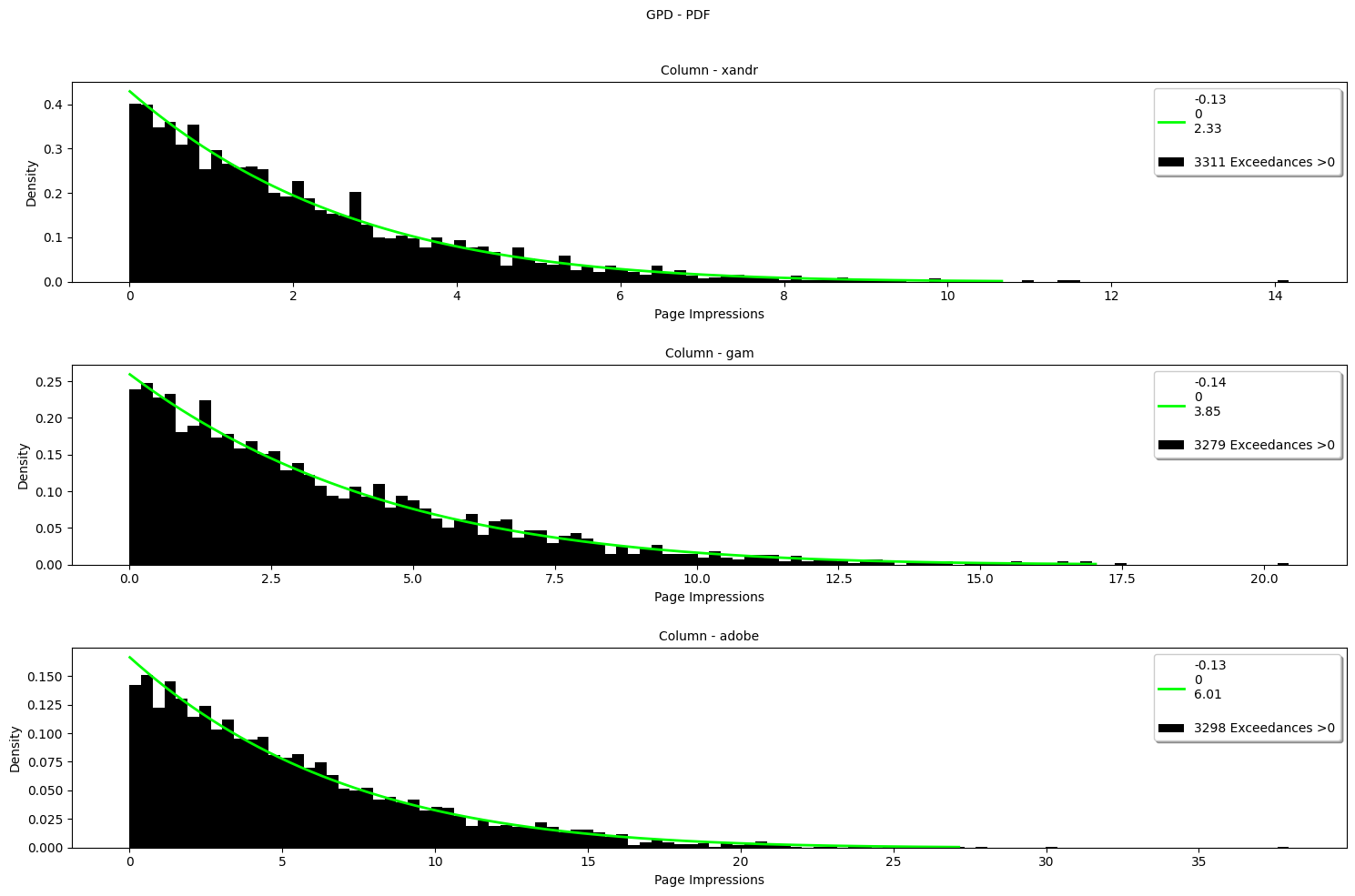
    7. Let’s inspect the GPD distributions to get the intuition of our pareto distribution:

      pot_detector.plot(ptype="hist-gpd-df", title="GPD - PDF", xlabel="Page Impressions", ylabel="Density", alpha=1.0, bins=100)

      GPD-PDF

    8. The parameters are stored inside the detector class:

      pot_detector.params
      {0: {'xandr': {'c': -0.11675297447288158,
      'loc': 0,
      'scale': 2.3129766056305603,
      'p_value': 0.9198385927065513,
      'anomaly_score': 1.0871472537998},
      'gam': {'c': 0.0,
      'loc': 0.0,
      'scale': 0.0,
      'p_value': 0.0,
      'anomaly_score': 0.0},
      'adobe': {'c': 0.0,
      'loc': 0.0,
      'scale': 0.0,
      'p_value': 0.0,
      'anomaly_score': 0.0},
      'total_anomaly_score': 1.0871472537998},
      1: {'xandr': {'c': 0.0,
      'loc': 0.0,
      'scale': 0.0,
      'p_value': 0.0,
      'anomaly_score': 0.0},
      'gam': {'c': 0.0,
      'loc': 0.0,
      'scale': 0.0,
      'p_value': 0.0,
      ...
      'scale': 0.0,
      'p_value': 0.0,
      'anomaly_score': 0.0},
      'total_anomaly_score': 0.0},
      ...}
    9. Last but not least, we can now detect the extremely large (high) anomalies:

      pot_detector.detect(0.95)
      pot_detector.detection_result
      16425    False
      16426    False
      16427    False
      16428    False
      16429    False
              ...
      22990    False
      22991    False
      22992    False
      22993    False
      22994    False
      Name: detected data, Length: 6570, dtype: bool
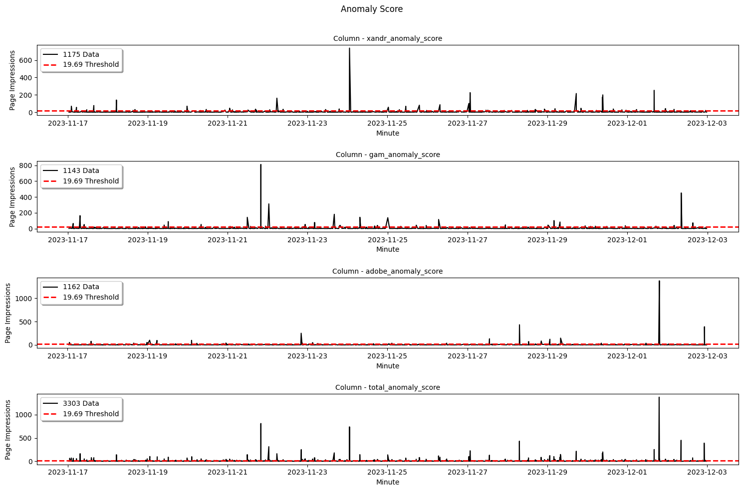
    10. Now we can visualize the anomaly scores from the fitting with the anomaly threshold to get the sense of the extremely large values:

      pot_detector.plot(ptype="line-anomaly-score-df", title="Anomaly Score", xlabel="Minute", ylabel="Page Impressions", alpha=1.0)

      Anomaly Scores

    11. Now what? Well, while the detection process seems quite straight forward, in most cases getting the details of each anomalous data is quite tidious! That’s why anomalytics provides a comfortable method to get the summary of the detection so we can see when, in which row, and how the actual anomalous data look like:

      pot_detector.detection_summary.head(5)
                                row	    xandr	      gam	    adobe	xandr_anomaly_score	gam_anomaly_score	adobe_anomaly_score	total_anomaly_score	anomaly_threshold
      2023-11-28 12:06:00	    59225	64.117135	76.425925	47.772929	          21.445759	        0.000000	          0.000000	          21.445759	        19.689885
      2023-11-28 12:25:00	    59244	40.513415	94.526021	65.921644	          0.000000	        19.557962	          2.685337	          22.243299	        19.689885
      2023-11-28 12:45:00	    59264	52.362039	54.191719	79.972860	          0.000000	        0.000000	          72.313273	          72.313273	        19.689885
      2023-11-28 16:48:00	    59507	64.753203	70.344142	42.540168	          32.543021	        0.000000	          0.000000	          32.543021	        19.689885
      2023-11-28 16:53:00	    59512	35.912221	52.572939	75.621003	          0.000000	        0.000000	          22.199505	          22.199505	        19.689885
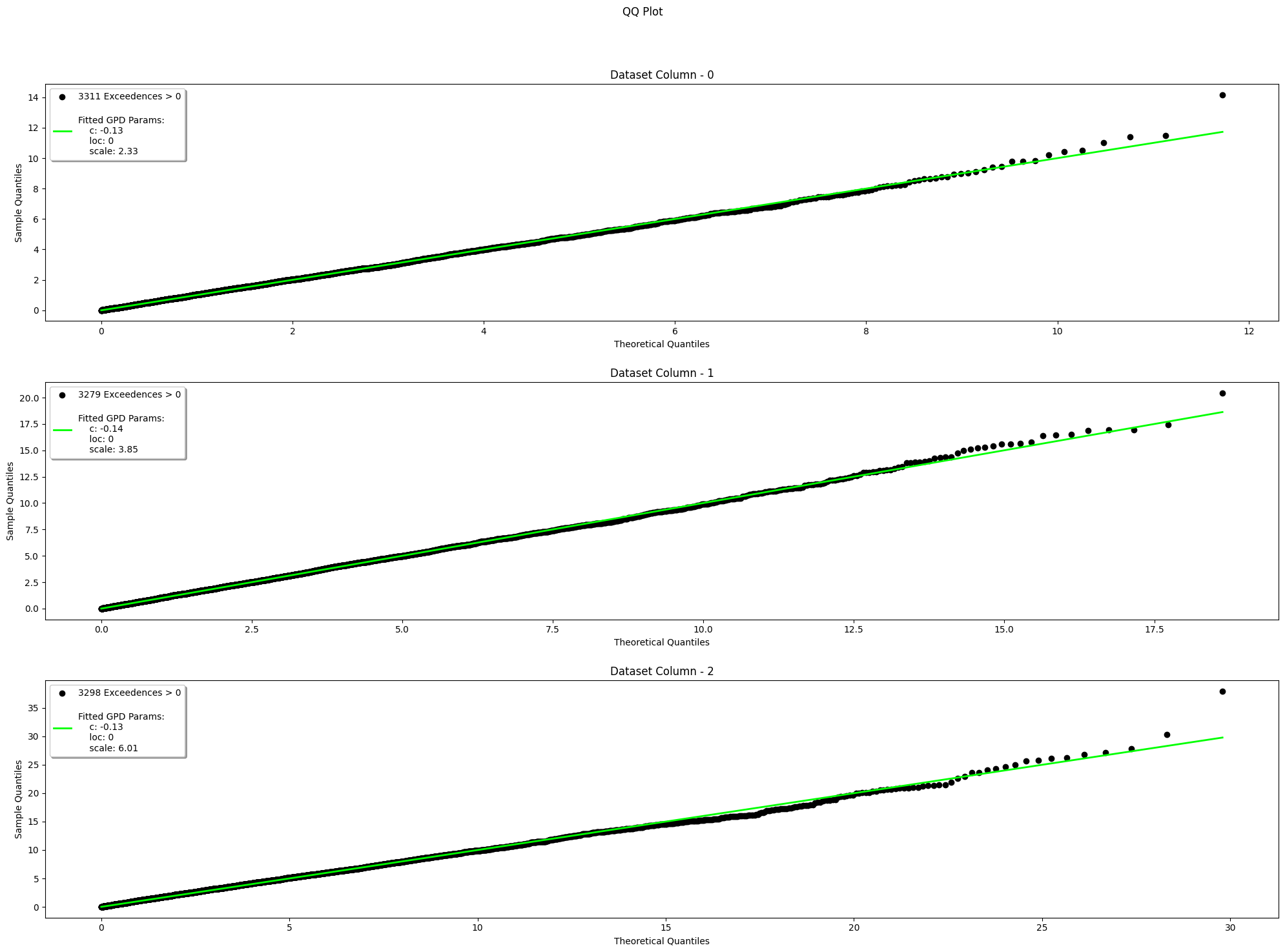
    12. In every good analysis there is a test! We can evaluate our analysis result with “Kolmogorov Smirnov” 1 sample test to see how far the statistical distance between the observed sample distributions to the theoretical distributions via the fitting parameters (the smaller the stats_distance the better!):

      pot_detector.evaluate(method="ks")
      pot_detector.evaluation_result
          column	total_nonzero_exceedances	stats_distance	p_value	        c	loc	    scale
      0	 xandr	                     3311	      0.012901	0.635246 -0.128561	  0	 2.329005
      1	 gam	                     3279	      0.011006	0.817674 -0.140479	  0	 3.852574
      2	 adobe	                     3298	      0.019479	0.161510 -0.133019	  0	 6.007833
    13. If 1 test is not enough for evaluation, we can also visually test our analysis result with “Quantile-Quantile Plot” method to observed the sample quantile vs. the theoretical quantile:

      # Use the last non-zero parameters
      pot_detector.evaluate(method="qq")
      
      # Use a random non-zero parameters
      pot_detector.evaluate(method="qq", is_random=True)

      QQ-Plot GPD

    Anomaly Detection via Standalone Functions

    You have a project that only needs to be fitted? To be detected? Don’t worry! anomalytics also provides standalone functions as well in case users want to start the anomaly analysis from a different starting points. It is more flexible, but many processing needs to be done by you. LEt’s take an example with a different dataset, thistime the water level Time Series!

    1. Import anomalytics and initialise your time series:

      import anomalytics as atics
      
      ts = atics.read_ts(
          "water_level.csv",
          "csv"
      )
      ts.head()
      2008-11-03 06:00:00    0.219
      2008-11-03 07:00:00   -0.041
      2008-11-03 08:00:00   -0.282
      2008-11-03 09:00:00   -0.368
      2008-11-03 10:00:00   -0.400
      Name: Water Level, dtype: float64
    2. Set the time windows of t0, t1, and t2 to compute dynamic expanding period for calculating the threshold via quantile:

      t0, t1, t2 = atics.set_time_window(
          total_rows=ts.shape[0],
          method="POT",
          analysis_type="historical",
          t0_pct=0.65,
          t1_pct=0.25,
          t2_pct=0.1
      )
      
      print(f"T0: {t0}")
      print(f"T1: {t1}")
      print(f"T2: {t2}")
      T0: 65001
      T1: 25001
      T2: 10000
    3. Extract exceedances and indicate that it is a "high" anomaly type and what’s the quantile:

      pot_thresholds = get_threshold_peaks_over_threshold(dataset=ts, t0=t0, "high", q=0.90)
      pot_exceedances = atics.get_exceedance_peaks_over_threshold(
          dataset=ts,
          threshold_dataset=pot_thresholds,
          anomaly_type="high"
      )
      
      exceedances.head()
      2008-11-03 06:00:00    0.859
      2008-11-03 07:00:00    0.859
      2008-11-03 08:00:00    0.859
      2008-11-03 09:00:00    0.859
      2008-11-03 10:00:00    0.859
      Name: Water Level, dtype: float64
    4. Compute the anomaly scores for each exceedance and initialize a params for further analysis and evaluation:

      params = {}
      anomaly_scores = atics.get_anomaly_score(
          exceedance_dataset=pot_exceedances,
          t0=t0,
          gpd_params=params
      )
      
      anomaly_scores.head()
      2016-04-03 15:00:00    0.0
      2016-04-03 16:00:00    0.0
      2016-04-03 17:00:00    0.0
      2016-04-03 18:00:00    0.0
      2016-04-03 19:00:00    0.0
      Name: anomaly scores, dtype: float64
      ...
    5. Inspect the parameters:

      params
      {0: {'index': Timestamp('2016-04-03 15:00:00'),
      'c': 0.0,
      'loc': 0.0,
      'scale': 0.0,
      'p_value': 0.0,
      'anomaly_score': 0.0},
      1: {'index': Timestamp('2016-04-03 16:00:00'),
      ...
      'c': 0.0,
      'loc': 0.0,
      'scale': 0.0,
      'p_value': 0.0,
      'anomaly_score': 0.0},
      ...}
    6. Detect anomalies:

      anomaly_threshold = get_anomaly_threshold(
          anomaly_score_dataset=anomaly_scores,
          t1=t1,
          q=0.90
      )
      detection_result = get_anomaly(
          anomaly_score_dataset=anomaly_scores,
          threshold=anomaly_threshold,
          t1=t1
      )
      
      detection_result.head()
      2020-03-31 19:00:00    False
      2020-03-31 20:00:00    False
      2020-03-31 21:00:00    False
      2020-03-31 22:00:00    False
      2020-03-31 23:00:00    False
      Name: anomalies, dtype: bool
    7. For the test, kolmogorov-smirnov and qq plot are also accessible via standalone functions, but the params need to be processed so it only contains a non-zero parameters since there are no reasons to calculate a zero 😂

      nonzero_params = []
      
      for row in range(0, t1 + t2):
          if (
              params[row]["c"] != 0
              or params[row]["loc"] != 0
              or params[row]["scale"] != 0
          ):
              nonzero_params.append(params[row])
      
      ks_result = atics.evals.ks_1sample(
          dataset=pot_exceedances,
          stats_method="POT",
          fit_params=nonzero_params
      )
      
      ks_result
      {'total_nonzero_exceedances': [5028], 'stats_distance': [0.0284] 'p_value': [0.8987], 'c': [0.003566], 'loc': [0], 'scale': [0.140657]}
    8. Visualize via qq plot:

      nonzero_exceedances = exceedances[exceedances.values > 0]
      
      visualize_qq_plot(
          dataset=nonzero_exceedances,
          stats_method="POT",
          fit_params=nonzero_params,
      )

    Sending Anomaly Notification

    We have anomaly you said? Don’t worry, anomalytics has the implementation to send an alert via E-Mail or Slack. Just ensure that you have your email password or Slack webhook ready. This example shows both application (please read the comments 😎):

    1. Initialize the wanted platform:

      # Gmail
      gmail = atics.get_notification(
          platform="email",
          sender_address="my-cool-email@gmail.com",
          password="AIUEA13",
          recipient_addresses=["my-recipient-1@gmail.com", "my-recipient-2@web.de"],
          smtp_host="smtp.gmail.com",
          smtp_port=876,
      )
      
      # Slack
      slack = atics.get_notification(
          platform="slack",
          webhook_url="https://slack.com/my-slack/YOUR/SLACK/WEBHOOK",
      )
      
      print(gmail)
      print(slack)
      'Email Notification'
      'Slack Notification'
    2. Prepare the data for the notification! If you use standalone, you need to process the detection_result to become a DataFrame with row, “

      # Standalone
      detected_anomalies = detection_result[detection_result.values == True]
      anomalous_data = ts[detected_anomalies.index]
      standalone_detection_summary = pd.DataFrame(
          index=anomalous.index.flatten(),
          data=dict(
              row=[ts.index.get_loc(index) + 1 for index in anomalous.index],
              anomalous_data=[data for data in anomalous.values],
              anomaly_score=[score for score in anomaly_score[anomalous.index].values],
              anomaly_threshold=[anomaly_threshold] * anomalous.shape[0],
          )
      )
      
      # Detector Instance
      detector_detection_summary = pot_detector.detection_summary
    3. Prepare the notification payload and a custome message if needed:

      # Email
      gmail.setup(
          detection_summary=detection_summary,
          message="Extremely large anomaly detected! From Ad Impressions Dataset!"
      )
      
      # Slack
      slack.setup(
          detection_summary=detection_summary,
          message="Extremely large anomaly detected! From Ad Impressions Dataset!"
      )
    4. Send your notification! Beware that the scheduling is not implemented since it always depends on the logic of the use case:

      # Email
      gmail.send
      
      # Slack
      slack.send
      'Notification sent successfully.'
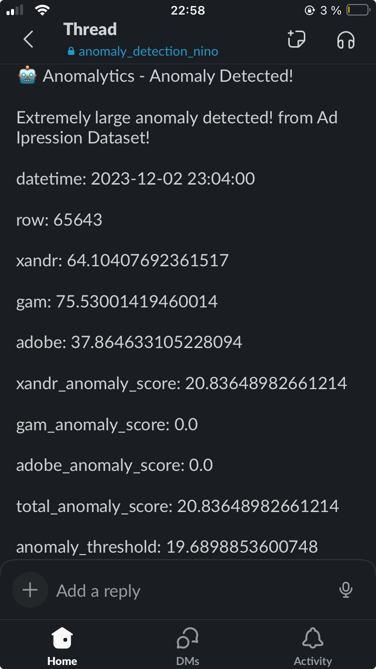
    5. Check your email or slack, this example produces the following notification via Slack:

      Anomaly SLack Notification

    Reference

    • Nakamura, C. (2021, July 13). On Choice of Hyper-parameter in Extreme Value Theory Based on Machine Learning Techniques. arXiv:2107.06074 [cs.LG]. https://doi.org/10.48550/arXiv.2107.06074

    • Davis, N., Raina, G., & Jagannathan, K. (2019). LSTM-Based Anomaly Detection: Detection Rules from Extreme Value Theory. In Proceedings of the EPIA Conference on Artificial Intelligence 2019. https://doi.org/10.48550/arXiv.1909.06041

    • Arian, H., Poorvasei, H., Sharifi, A., & Zamani, S. (2020, November 13). The Uncertain Shape of Grey Swans: Extreme Value Theory with Uncertain Threshold. arXiv:2011.06693v1 [econ.GN]. https://doi.org/10.48550/arXiv.2011.06693

    • Yiannis Kalliantzis. (n.d.). Detect Outliers: Expert Outlier Detection and Insights. Retrieved [23-12-04T15:10:12.000Z], from https://detectoutliers.com/

    Wall of Fame

    I am deeply grateful to have met and guided by wonderful people who inspired me to finish my capstone project for my study at CODE university of applied sciences in Berlin (2023). Thank you so much for being you!

    • Sabrina Lindenberg
    • Adam Roe
    • Alessandro Dolci
    • Christian Leschinski
    • Johanna Kokocinski
    • Peter Krauß
    Visit original content creator repository https://github.com/Aeternalis-Ingenium/anomalytics